What is a Single Variable Linear Regression and how to Carry Out it in Excel and in R

The R code could be found on: https://github.com/FranciscoRiano/r_data_visualization_n_analysis

A single variable linear regression is a statistical methodology that allows us to assess the magnitude of a relationship between two variables and make forecasts based on a linear equation. This linear equation is:  where:

• Y represents the dependent variable for a given x value
• X is the independent value
• A is the intercept. It represents the value of y when the independent variable x is equal to 0
• B is the slope. It is the average change in the dependent variable y as the independent variable x increases by 1. When the slope is 0, it means that does not exist any relationship between the assessed variables

As soon as we were able to determine the linear equation, we will just have to replace the values in order to get the dependent variable y forecasted value. It is also possible to build prediction interval, an interval which is likely to contain the forecasted value.

Besides the linear equation parameters, it is also important to analyze other elements that are fundamental in order to understand the quality of our model and the strength of the relationship between the two studied variables. These elements are:

• R or correlation coefficient: Basically, is the degree of relationship between the dependent y and independent x variables. It can go between -1 to 1. When this measure is negative, it means that the two variables have an inversely proportional relationship. When it goes close to 0 it means that the relationship is irrelevant and when it gets closer to 1 it indicates a proportional relationship.
• R^2: it measures the rate of the variation in the dependent y variable that is explained by the model. It means that the higher this indicator, the better our model is, or at least the better that our model explain the variation in the dependent y variable. It goes from 0 to 1 or 0% to 100%. Just for single variable linear regression models, this measure is equal to the square of the correlation coefficient
• P-value: This metric test whether there is a significant linear relationship between the two variables. In deeper terms the p-value says the probability that the slope is equals to 0. If the slope is equals to 0 that means that does not exist at all any relationship between the two variables. Bearing in mind this, it is possible to conclude that the smaller the p-value, the stronger the relationship between the two variables.

Once we have seen what is a single variable linear regression with a theorical approach, now it is time to see how to apply it in Excel and more important how to interpret the result with a business approach. For this exercise one dataset downloaded from Kaggle has been used. This data is from houses with different features such as: price, year of construction, size, number of bathrooms, bedrooms etc. It is clear that the price of a house is determined by several variables, however just to simplify the exercise I have done it just with two variables.

In order to create a single variable linear regression in Excel, first what we have to do is to go to the ribbon and select the Data menu. Then we will have to choose the Data Analysis option

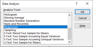
After that we will see a menu that will allow us to select from several option in order to analyze our data. We will choose the Regression option in order to carry out the model.

After that, Excel is going to allow us to select both, the dependent y variable and the independent x variable. Also, we are going to be able to modify other features such as the sheet where we want to get deployed the summary, or if the selected data range has labels or not.

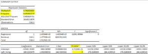
This is the summary generated once we fix up all the require parameters. It is important to get focused initially in the three variables explained before.

First it is important to realize that this summary generated in Excel calls the correlation coefficient as Multiple R. As we can see, in this case the correlation coefficient is 0.70 or for practical purposes 70%. It means that the strength of the linear relationship between the two selected variables (price of the houses as dependent variable and size as independent variable) in quantitative terms correspond to a 70% which is quite acceptable.

Let’s go forward with the p-value. Let’s recall that the p-value is the probability that the slope is equal to 0, let’s also remember that if the slope is 0 that means that there is not any relationship between the two selected variables. Given that in our exercise p-value is equal to 0, that means that definitely there is a linear relationship between the two variables.

Let’s recall that the R square is the square of the correlation coefficient. In this case given that the correlation coefficient is 70% so our R square corresponds to a 49%. It means that in a rate of 49% our model explains the variation in the dependent y variable.

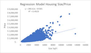
In order to distinguish much better the differences between the interpretation given to the R square and the p-value, let’s see the scatter plot graph of the model. As we can see all the points are relatively congregated to each other. If we would have got a different model, with the same p-value but with a lower R square value, it would have the points much more scattered along the graph.

Until now we have done the whole exercise through Excel but, given that the features of the Excel plotter are relatively limited, what if we use a complement in order to explain much better our model even including new variables? In this case we are going to use RStudio to carry out it.

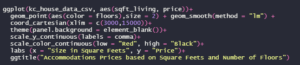
In our first example using R, we are going to create again a scatter plot but this time with more details and items that are important in order to understand our model and analysis with just one glance.

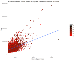
For instance, this scatter plot graph seems exactly the same as the one created in Excel, however in this case we have included a third variable that is the number of floors. So, although this chart says exactly the same as the one created in Excel, now it is possible to watch also the influence of a third variable on the analysis. This scatter plot in R has been created with the following code:

A graph that also could be a huge aid in this exercise is the histogram. We can use the following code to get that histogram:

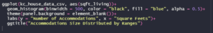
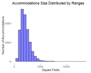
With the previous code we are going to create the following histogram:

If we want to get the single variable regression summary in R it is also possible to get it just through one code line that is:

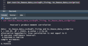
The highlighted line is the code itself and the information at the bottom of the picture is the summary. We will see that this information matches completely with the summary got from Excel.

After we have seen what a single variable linear regression means and its importance to get relevant insights in any business context, it is possible to conclude that this theorical and practical framework should be adopted by any organization in order to reduce risks, make better forecasts and to get better sights and analysis of the data.